SimuLab 7: Average Position after N Steps
How far from the origin does the wandering ant end up after some number (N) of steps? What do you guess: after 10 steps is the walker more likely to be to the right or to the left of its starting point? If another ant takes 10 steps from the starting point, then another ant, then another ant, what do you expect their average final position to be after 10 steps?
Investigate! Go back to the ManyWalkers program and observe the value of "AVG. x'' given at the right of the bar graph. The symbol x stands for the number of steps a walker is displaced from the initial position. The value of x is positive if displacement is to the right, negative if to the left. How does this average change as the number of steps increases? Is AVG. x bigger for more walkers? Or is it smaller for more walkers? Press the Store button to record any interesting set of averages; then press the Table button to examine the data you have saved.
What does theory have to say about the value of the average position of many random walkers? Here we are not talking about averaging a small number of walkers: not 100 walkers, not 1000 walkers, not even one million walkers. We ask: What is the average position of an infinite number of walkers? Answer: The value of the average position is zero, the position of the starting point (the lamp post)! How can this be? One word gives the reason: Symmetry! In this case symmetry means that moving right is just as likely as moving left. After any fixed number of steps, the walker is equally likely to be to the right of the starting point (positive displacement) as to the left (negative displacement). Moreover, for a given number of steps, the distance x from the starting point is likely to have the same value, whether displacement is to the right (positive x) or to the left (negative x). In brief, averaged over many millions of trials, the positive displacements cancel the negative displacements. Therefore we expect the average of many trials to be zero; the average position of the walkers is at the starting point.
The average position may be zero, but the spread of positions is not zero, as shown also by the examples in Figures 3.5 and 3.6. The number of heads in 10 trials does not always come out the same. The number of heads can vary in each 10-step trial.
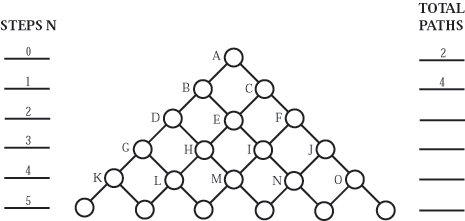
How can this spread of final positions be described? Pascal's Triangle helps to answer this question. Look at the Pascal Triangle shown in Figure 3.7 We are going to do something that turns out to be very useful: Count the number of paths that can lead to each of the pegs in the 2nd row, the 3rd row, the 4th row, etc.
 |
The first two rows are done already. For example, the only way to get to point D (after 2 steps) is by going left-left (LL). We enter a 1 in circle D, meaning there is only one way to get there. In contrast, there are two alternative paths to point E, namely left-right (LR) or right-left (RL). Therefore we enter the number 2 in circle E. How many paths are there to point F? Now you fill in the next two rows. You need 3 steps and 4 steps to reach the pegs in these rows, respectively.
Now we state a very important rule. Starting from some initial point, and for a random choice at each step
| every alternative path to a given final point is equally likely. |
In other words, two paths are alternative -or different
-if any segment of one path is different from that of
the other path.
As an example of the new rule, look at row 3, where the ball arrives after two steps. There are two paths to central position E, but only one path to each of the end positions D and F. The rule above says that a random walker is twice as likely to end up at the central position E than at either of the positions D or F.
Is this rule reasonable? We have assumed that as the ball comes to each peg, it is equally likely to fall to the left of the peg as to the right. And every possible path is made up of a sequence of these equal choices. So it is reasonable that every path to a given final point is as likely as every other possible path to that point.
It
is easy to find a rule that allows us to determine how many (equally
likely!) paths lead to a given peg in Pascal's Triangle: The number
in each circle is the sum of the numbers in the two adjacent circles
above it in the previous row. (For the end circles, the number is
the same as in the one adjacent circle in the row above.)
For example, the number in circle E is 2, equal to the sum of the
numbers 1+1 in circles B and C above it. Is this reasonable? Think
of paths. There is 1 possible path leading into B, one possible
path leading into C. Therefore they provide
|
Use this rule to make entries in the circles of rows 3 and 4 in a copy of Figure 3.7. Also put numbers in the circles for the fifth row at the bottom of the figure.
If every alternative path is equally likely, then the more paths that lead to a given peg, the more likely the ball is to arrive at that peg. For example, two paths lead to peg E in Figure 3.7, while only one path leads to each of pegs D and F in the same row. The total number of paths that arrive in that row are 1+2+1 = 4 (number at the right side of the figure). The probability that a ball arrives at peg E is 2/4 = 1/2. A similar analysis can be applied to a peg in any row of Figure 3.7.
Using Pascal's Triangle, we have described the number of different paths (and relative likelihood, that is, probability) of arriving at any location (at any circle in the diagram) after a certain number of steps. The result is too many numbers. It is time to simplify our picture by using averages.
Previous: SimuLab 6 - Width of a Distribution